Solving Large-Scale Warehouse Optimization: From MILP to Column Generation

Imagine a warehouse with thousands of trays arriving daily. Your task is to arrange them into neat lanes, but there's a catch: you need to use as few lanes as possible to save floor space, while also keeping each lane short enough for your forklifts to operate efficiently. This is a classic large-scale optimization puzzle where off-the-shelf solvers can grind to a halt. In this post, we'll explore how to model this challenge, starting with a standard mathematical formulation and escalating to a powerful technique called Column Generation, designed specifically for problems of this scale.

we can view this as a sophisticated variant of the classic Bin Packing Problem. In the standard problem, you minimize the number of bins. Here, we have a trickier, bi-objective goal: we want to minimize the number of 'bins' (lanes) and minimize the length of the longest 'bin'.

What is a bin packing problem?

Bin packing problem is a classic optimization problem where you have a set of items and a set of bins, and you want to pack the items into the bins such that the total volume of the items is less than or equal to the volume of the bins.

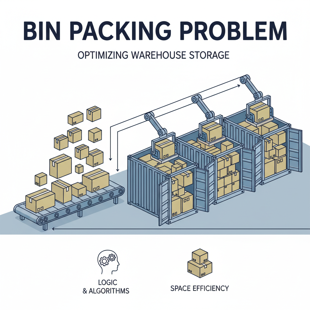
According to Wikipedia, the bin packing problem is a combinatorial optimization problem where the goal is to pack a set of items into a finite number of bins or containers, minimizing the number of bins used while satisfying certain constraints. The items are typically of different sizes, and the bins have a fixed capacity. The problem is NP-hard, meaning that no efficient algorithm is known for solving it optimally in polynomial time.

A practical-alike example

Currently, imagine you store trays in a linear lane system positioned against a wall in one corner of the facility. Each lane extends perpendicular from the wall and accommodates trays in a single-file arrangement. While you initially considered stacking trays to maximize vertical space, safety concerns led us to maintain single-level storage.

The standard lane configuration calls for:

1-meter lane width
1.9-meter maximum lane length

However, real-world operations often require us to exceed these parameters. When daily tray volumes don't fit within our ideal dimensions, we face two scenarios: lanes that stretch beyond 2 meters, or an increased number of lanes. While both solutions are workable, they create challenges for our forklift operators who need clear, straight pathways perpendicular to the storage lanes.

Additionally, our trays come in three distinct sizes—Small, Medium, and Large—each with fixed dimensions that must be oriented in a specific direction within the lanes due to handling requirements.

Mathematical formulation

First, we define the following sets and parameters, decision variables, objective function, and constraints for the problem.

I = \{1, 2, \ldots, n\} \quad \text{(set of trays)}

J = \{1, 2, \ldots, m\} \quad \text{(set of available lanes)}

\alpha \in [0,1] \quad \text{(weight parameter for bi-objective function)}

$\ell_i$ denotes the length for tray $i$ .

For decision variables, we have:

x_{ij} = \begin{cases} 1 & \text{if tray } i \text{ is assigned to lane } j \\ 0 & \text{otherwise} \end{cases} \quad \forall i \in I, j \in J

y_j = \begin{cases} 1 & \text{if lane } j \text{ is used} \\ 0 & \text{otherwise} \end{cases} \quad \forall j \in J

z \geq 0 \quad \text{(maximum lane length)}

s_j \geq 0 \quad \text{(length of lane } j\text{)} \quad \forall j \in J

We have the following objective function:

\min \quad \alpha z + (1 - \alpha) \sum_{j=1}^{m} y_j

The objective function balances two competing goals:

Minimize the maximum lane length
Minimize the number of lanes used

We also have the basic constraints for the problem:

Unique assignment: Each tray is assigned to exactly one lane.

\sum_{j=1}^{m} x_{ij} = 1 \quad \forall i \in I

Lane length definition: The length of each lane equals the sum of assigned tray lengths.

s_j = \sum_{i=1}^{n} \ell_i x_{ij} \quad \forall j \in J

Lane usage constraint: Lane usage is activated when trays are assigned.

\sum_{i=1}^{n} x_{ij} \leq M\times y_j \quad \forall j \in J

This is the Big-M constraint and we define $M = n$ in our problem.

Maximum lane length definition: Define the maximum length across all lanes.

z \geq s_j \quad \forall j \in J

Feasibility: At least one lane must be used.

\ell_i \leq z \quad \forall i \in I

This constraint ensures that the maximum lane length z is at least as large as the longest single tray, which is a logical lower bound.

Variable Domains:

x_{ij} \in \{0, 1\} \quad \forall i \in I, j \in J

y_j \in \{0, 1\} \quad \forall j \in J

z, s_j \geq 0 \quad \forall j \in J

Sensitivity analysis

Sensitivity analysis is a technique used to understand how changes in the input parameters of a model affect the output. In our problem, we can perform sensitivity analysis on the weight parameter $\alpha$ .

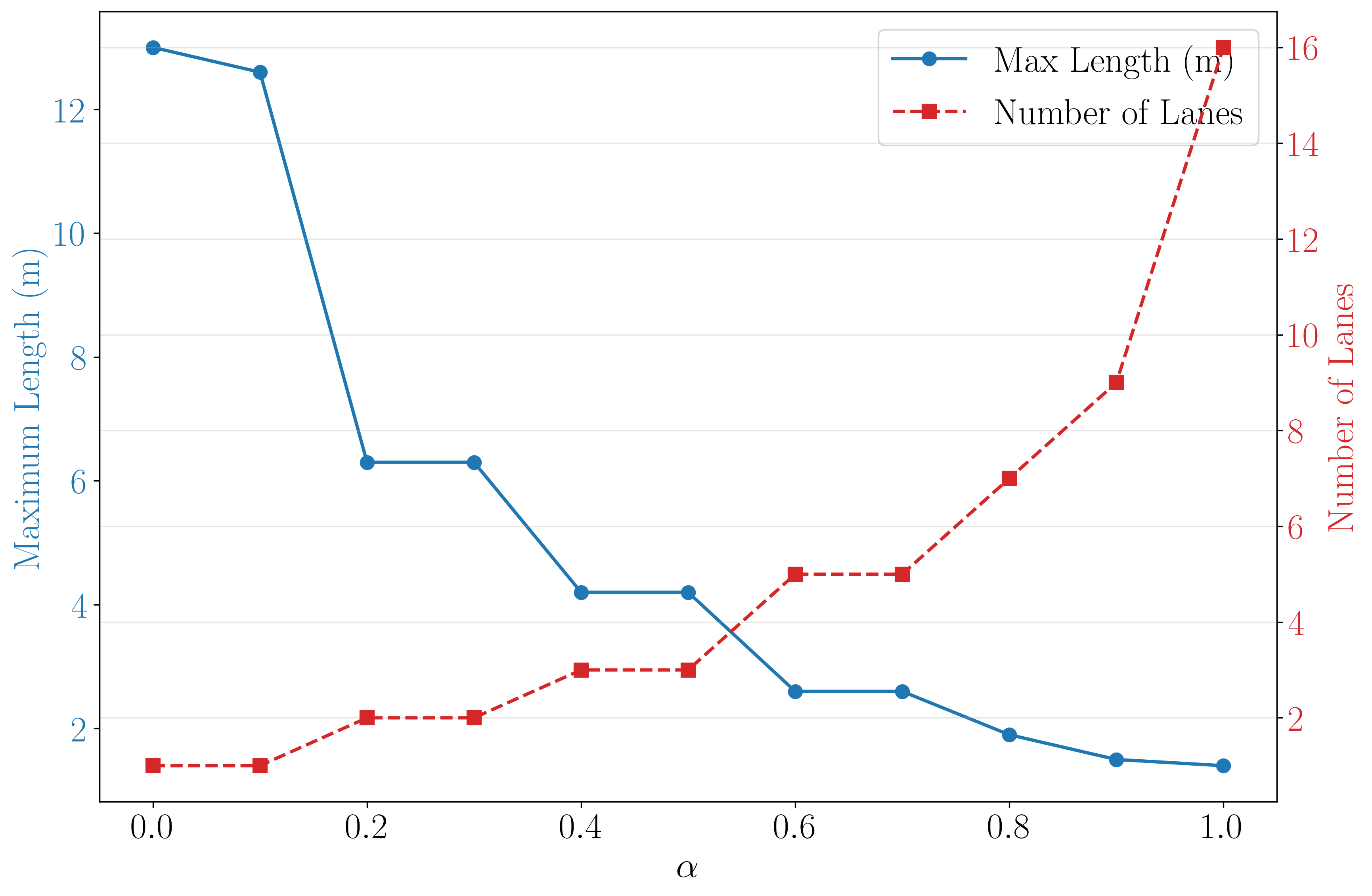
The figure illustrates that the trade-off is unavoidable: as we reduce the number of lanes (red line going down), the maximum lane length must increase (blue line going up). The practical decision comes down to what matters more operationally: minimizing the number of lanes (to save floor space) or keeping lanes shorter (for forklift efficiency).

It's easy to present this chart to stakeholders and ask the following business question: ``Given your forklift operations and available floor space, which part of the figure represents the best compromise for your daily operations?" If the idea length for the lane is equal or lower than 2 meters, the number of lanes will be at least 7 (according to the 16 tray testing). This gives them a visual tool to make informed decisions based on their specific operational priorities rather than leaving it as an abstract optimization problem.

Scaling Up: When MILP Hits a Wall, Enter Column Generation

The MILP formulation is clear and exact. For a few dozen trays, it works beautifully. But what happens when you have 700, 1,000, or 10,000 trays? The number of possible assignments ( $x_{ij}$ ) is $2^{n}$ for each tray $i$ , which is prohibitively large. Using this problem as an example, even with advanced MILP tricks like symmetry breaking constraints, and variable fixing strategies, the problem becomes intractable.

This is a classic symptom of a problem perfectly suited for Column generation. The core idea of CG is to change our perspective. Instead of thinking about assigning individual trays to lanes (a massive number of decisions), we think about building a library of "good" lane configurations, called patterns. Then, our only decision is how many times to use each pattern from our library. We don't need to know every possible pattern in the universe to start. We can start with a few obvious ones and then intelligently generate new, better patterns only when we need them. This is the magic of column generation: it avoids getting lost in a sea of possibilities by only considering the most promising ones.

The New Structure: A Master Problem and a Pricing Subproblem

The CG approach splits the problem into two coordinated parts:

The Master Problem: This is the manager. It looks at the current library of known patterns and tries to find the best way to combine them to satisfy all the tray requirements at the minimum cost. It's a relatively small and easy-to-solve problem.
The Pricing Subproblem (or "Pattern Generator"): This is the creative expert. The Master Problem asks the Subproblem a crucial question: "Given my current costs, can you find a new, unlisted pattern that would improve my overall solution?" These two problems "talk" to each other in a loop until the Subproblem can no longer find any better patterns.

The Master Problem: Choosing the Best Patterns

Let's formalize the manager's task. We define a "pattern" as a valid combination of trays that can fit into a single lane. The Sets and Parameters are as follows:

I = \{1, 2, \ldots, n\} \quad \text{(set of trays)}

P = \{1, 2, \ldots, |P|\} \quad \text{(set of feasible patterns)}

\alpha \in [0,1] \quad \text{(weight parameter for bi-objective function)}

For each pattern $p \in P$ :

$T_p \subseteq I$ : set of trays included in pattern $p$
$L_p = \sum_{i \in T_p} \ell_i$ : total length of pattern $p$
$a_{ip} = \begin{cases} 1 & \text{if tray } i \text{ is in pattern } p \\ 0 & \text{otherwise} \end{cases}$

Decision Variables:

\lambda_p \geq 0 \quad \text{(number of times pattern } p \text{ is used)} \quad \forall p \in P \\

z \geq 0 \quad \text{(maximum lane length)}

Objective Function:

\min \quad \alpha z + (1 - \alpha) \sum_{p \in P} \lambda_p

Constraints:

Tray coverage: Each tray must be covered exactly once

\sum_{p \in P} a_{ip} \lambda_p = 1 \quad \forall i \in I

Maximum length definition:

L_p \lambda_p \leq z \quad \forall p \in P

Variable domains:

\lambda_p \geq 0 \quad \forall p \in P, \quad z \geq 0

This is a Linear Program (LP), which is very fast to solve. When we solve it, we get two crucial pieces of information: the current best solution $\lambda_p^*$ and the dual values. The dual values are the shadow prices of the constraints. A higher dual value means the Master Problem is struggling to place tray $i$ and would pay a high price for a pattern that includes it.

The Pricing Subproblem: Finding a Better Pattern

Let $\pi_i$ be the dual variable for Tray coverage constraint and $\sigma_p$ be the dual variable for Maximum length definition constraint. The pricing subproblem finds the pattern with the most negative reduced cost. The subproblem's goal is to use the prices ( $\pi_i$ and $\sigma_p$ ) from the Master Problem to find a new pattern that is a "good deal."

Decision Variables:

x_i = \begin{cases} 1 & \text{if tray } i \text{ is included in the new pattern} \\ 0 & \text{otherwise} \end{cases} \quad \forall i \in I

Objective Function:

Maximize the reduced cost:

\max \quad \sum_{i \in I} \pi_i x_i - (1 - \alpha)

The term $(1 - \alpha)$ represents the coefficient of $\lambda_p$ in the master problem objective.

Constraints:

Length feasibility: Pattern must fit in a lane

\sum_{i \in I} \ell_i x_i \leq L_{\text{max}} \tag{SP1}

Compatibility constraints: Large and medium trays cannot coexist

x_i + x_j \leq 1 \quad \forall i \in I_{\text{large}}, j \in I_{\text{medium}} \tag{SP2}

where $I_{\text{large}}$ and $I_{\text{medium}}$ are the sets of large and medium tray indices, respectively.

Variable domains:

x_i \in \{0, 1\} \quad \forall i \in I

This subproblem is a variation of the Knapsack Problem, which is NP-hard but can be solved very quickly for the sizes we care about.

The Column Generation Procedure: A Dialogue

The overall algorithm is an iterative conversation:

Initialize: Start with a simple set of patterns $P'$ (e.g., one pattern for each tray by itself). This guarantees a feasible, if terrible, starting solution.
Master Solves: Solve the Master Problem LP using the current set of patterns $P'$ . Get the dual prices $\pi_i$ .
Master Asks Subproblem: The Master sends the prices $\pi_i$ to the Subproblem and asks, "Can you find a new pattern with a negative reduced cost based on these prices?"
Subproblem Answers:
- If YES: The Subproblem solves its knapsack problem. If the optimal objective value is greater than 0 (meaning the reduced cost is negative), it has found a profitable new pattern. This pattern (defined by the x_i variables) is sent back to the Master. The Master adds this new "column" to its set $P'$ and goes back to Step 2.
- If NO: If the Subproblem's optimal objective value is 0 or less, it means no profitable pattern exists anywhere in the universe. The conversation is over. We have found the optimal solution to the LP relaxation.
Get the Final Integer Solution: Once the loop terminates, we have a great collection of highly effective patterns in $P'$ . We solve the Master Problem one last time, but now with the additional constraint that the variables $\lambda_p$ must be integers. This gives us our final, practical warehouse plan.

The Payoff: Solving the Unsolvable

After implementing this advanced approach, the computational improvements were dramatic. While the original MILP struggled with $n=700$ trays, the column generation algorithm delivered outstanding performance:

For an instance with $n=500$ trays, we found a solution with an optimality gap of just 0.38%, which is excellent for practical purposes.
A large instance with $n=1000$ trays was solved in 60.46 seconds.
A massive instance with $n=10000$ trays was solved in just 131.58 seconds.

This demonstrates the power of column generation: by reframing the problem and intelligently exploring the solution space, we can solve enormous, real-world instances that are completely out of reach for standard methods.

Key takeaways

Model the Real Problem: Many real-world optimization problems are variants of textbook cases. Don't be afraid to add custom constraints (like tray compatibility) to a standard model like Bin Packing to reflect operational reality.
From Math to Decisions: An optimization model's true value is unlocked when it's used as a decision-making tool. A sensitivity analysis chart is often more powerful for a stakeholder than a single "optimal" number.
Scale Kills, Advanced Methods Save: Standard MILP models are excellent, but their performance can degrade rapidly with size. For large-scale problems, advanced techniques like Column Generation are not just academic exercises—they are practical necessities for finding high-quality solutions in a reasonable timeframe.
The CG Mindset: Column Generation fundamentally reframes the problem from "assign items to bins" to "find the best combinations of items (patterns) and then choose from those." This "pattern-based" approach is a powerful paradigm for solving many large-scale combinatorial problems.